


ANUCLIM can also use climate surfaces to generate bioclimatic parameters for modelling species distributions, and to generate growth indices for modelling growth of crops and plants.
The supplied climate surfaces are location and topographic dependent functions that describe the spatial distribution of monthly mean values of daily minimum temperature, daily maximum temperature, precipitation, solar radiation, pan evaporation and others. These surfaces have been built using ANUSPLIN (Hutchinson 2004).
ANUCLIM consists of four programs - MTHCLIM, BIOCLIM, BIOMAP and GROCLIM. Each of these programs depends on the supplied climate surfaces and can incorporate climate change grids.
User guide
Download the ANUCLIM version 6.1 user guide (pdf, 1.9MB)
Features
ANUCLIM Version 6.1 incorporates substantial upgrades to the operation and flexibility of the package. In particular, it now allows for the systematic incorporation of climate change grids to enable the investigation of the impacts of projected climate change.
Other features include:
- Flexible grid-based climate change options available for all components of ANUCLIM.
- There are now two sets of Australian monthly mean climate surfaces for periods 1921-1995 and 1976-2005. Surfaces for additional time periods are anticipated.
- ESOCLIM renamed to MTHCLIM to better represent its function.
- Spatial discontinuities along the edges of precipitation surface tiles have been removed.
- Additional coordinate systems, including Lambert conformal conic, now supported.
- The bcp file produced by BIOMAP now records the user’s coordinate system.
- Naming convention of output files has been systematically revised to aid interpretation.
- No limit on the number of output files from GROCLIM.
- Special conditions on rainfall of driest period and driest quarter have been removed.
- Integer outputs have been replaced by real numbers with higher precision.
- The core Fortran programs have been substantially revised to be faster and more robust and all known bugs have been removed.
- Contents of output log files and warning messages have been revised to aid interpretation.
- The Graphical User Interface (GUI) has been revised to improve its operation and visual appearance.
Specifications
MTHCLIM
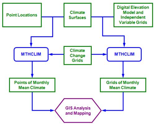
MTHCLIM is used to obtain estimates of monthly, seasonal and annual mean climate variables from the supplied monthly mean climate surfaces at specified points and grids. The locations of the points can be supplied either as a list of horizontal and elevation coordinates or as a regular grid, as supplied by a digital elevation model (DEM). A 9 second DEM for Australia is available from Geoscience Australia (ANU Fenner School of Environment and Society and Geoscience Australia, 2008).
For more information see the diagram of the main data flows for MTHCLIM.
BIOCLIM and BIOMAP
BIOCLIM, in conjunction with BIOMAP, is a bioclimatic prediction system originally devised by Nix (1986). The system uses bioclimatic parameters to gauge energy and water balances at given locations and employs a bioclimatic envelope method to predict the potential spatial distribution of species beyond known sample sites. BIOCLIM generates bioclimatic parameters from the supplied climate surfaces at known habitat locations for a particular plant or animal species. These parameters are then used to construct a bioclimatic profile (or bioclimatic envelope) for the species. As for MTHCLIM, BIOCLIM can output the bioclimatic parameters in point form, as calculated for a list of species habitat locations, and in regular grid form as calculated for a DEM. Error detection and correction, usually by examining and removing outliers in the bioclimatic profile, is an essential step in generating reliable bioclimatic predictions.
BIOMAP uses the species bioclimatic profile and grids of bioclimatic parameters calculated by BIOCLIM to predict the spatial distribution of the species. It does this by comparing the bioclimatic parameters at each grid location to the species bioclimatic profile generated by BIOCLIM. The impacts of projected climate change on predicted distributions are normally generated by applying climate change grids to the grids of bioclimatic parameters calculated by BIOCLIM.
For more information see the diagram of the main data flows for BIOCLIM and BIOMAP.
GROCLIM
GROCLIM is a simple generalised growth model of crop response to light, thermal and water regimes (Fitzpatrick and Nix 1970, Nix 1981) and is an extension of the program GROWEST (Hutchinson et al. 2004). It calculates weekly indices of light, temperature, moisture and growth for up to four different plant types from supplied climate surfaces at given locations. As for MTHCLIM, these locations can be calculated in the form of a list of sites or as a regular grid.
For more information see the diagram of the main data flows for GROCLIM.
Climate surfaces
Monthly mean climate surfaces are required to run MTHCLIM, BIOCLIM and GROCLIM. Australian monthly mean climate values are available for two nominated standard periods, 1921-1995 and 1976-2005. The 1976-2005 period is nominally centred on 1990, a standard baseline used for climate change assessments by the international scientific community.
ANUCLIM users outside Australia may need to calculate their own climate surfaces using the ANUSPLIN (Hutchinson 1991, 1995, 2004). The climate surfaces consist of a set of coefficient files that are used to generate interpolated climate values at specified locations. These coefficient files are produced by using the ANUSPLIN package from recorded monthly mean climate values at meteorological stations. These surfaces depend on location and topography.
Climate change grids
ANUCLIM Version 6.1 has been extensively upgraded to permit the application of flexible grid-based climate change scenarios. These scenarios can now be applied to all components of the ANUCLIM package. The climate scenarios can be defined either by simply providing constant change fields from the ANUCLIM Graphical User Interface or, more commonly, by supplying change grids.
The climate change grids must be supplied by the user. Temperature change grids are applied as additive changes. For non-negative climate variables, such as precipitation and pan evaporation, the change grids are applied as percentage changes. For Australia, climate change grids for a wide range of General Circulation Models (GCMs) and greenhouse gas emission scenarios can be downloaded from the OzClim website of CSIRO Australia. The climate change grids should have either the FLOATGRID or ASCIIGRID format of ESRI ArcGIS in order to be read by ANUCLIM Version 6.1 and must be in the geographic (longitude/latitude) coordinate system.
References
- ANU Fenner School of Environment and Society and Geoscience Australia, 2008. GEODATA 9 Second DEM and D8 Digital Elevation Model and Flow Direction Grid, User Guide (PDF 1MB). Geoscience Australia, 43 pp.
- Fitzpatrick, E.A. and Nix, H.A. 1970. The climatic factor in Australian grassland ecology. In: R. Milton Moore (ed), Australian Grasslands, Australian National University Press, Canberra.
- Hutchinson, M.F. 1991. The Application of thin plate smoothing splines to continent wide data assimilation. In: Data Assimilation Systems, J.D.Jasper (ed), Bureau of Meteorology Res. Rep. No. 27, Bureau of Meteorology, Melbourne, pp. 104113.
- Hutchinson, M.F. 1995. Interpolating mean rainfall using thin plate smoothing splines. International Journal of GIS 9: 385-403.
- Hutchinson, M.F. 2004. ANUSPLIN Version 4.3. Fenner School of Environment and Society, Australian National University, Canberra.
- Hutchinson, M.F., 2008. Adding the Z-dimension, In: J.P. Wilson and A.S. Fotheringham (eds), Handbook of Geographic Information Science, Blackwell, pp 144-168.
- Hutchinson, M.F. 2011. ANUDEM Version 5.3. Fenner School of Environment and Society, Australian National University, Canberra.
- Hutchinson, M.F., Booth, T.H., McMahon, J.P. and Nix, H.A. 1984. Estimating monthly mean values of daily total solar radiation for Australia, Solar Energy 32: 277‑290.
- Hutchinson, M.F. and Dowling,T.I. 1991. A continental hydrological assessment of a new gridbased digital elevation model of Australia. Hydrological Processes 5: 4558.
- Hutchinson, M.F., Kalma, J.D. and Johnson, M.E. 1984. Monthly estimates of windspeed and windrun for Australia, Journal of Climatology 4: 311‑324.
- Hutchinson, M.F., Nix, H.A., McMahon, J.P. and Ord, K.D. 1996. The development of a topographic and climate database for Africa. In: Proceedings of the Third International Conference/Workshop on Integrating GIS and Environmental Modeling, NCGIA, Santa Barbara, California.
- Hutchinson, M.F., Nix, H.A. and McTaggart, C. 2004. GROWEST Version 2.0. Fenner School of Environment and Society, Australian National University, Canberra.
- Kesteven, J.L. and Hutchinson, M.F. 1996. Spatial modelling of climatic variables on a continental scale. In: Proceedings of the Third International Conference/Workshop on Integrating GIS and Environmental Modeling, NCGIA, Santa Barbara, California.
- Nix, H.A. 1981. Simplified simulation models based on specified minimum data sets: the CROPEVAL concept. In: A. Berg (ed), Application of Remote Sensing to Agricultural Production Forecasting, Commission of the European Communities, Rotterdam, pp 151-169.
- Nix, H.A. 1986. A biogeographic analysis of Australian Elapid Snakes. In. Atlas of Elapid Snakes of Australia. (ed.) R. Longmore pp. 415. Australian Flora and Fauna Series Number 7. Australian Government Publishing Service: Canberra.
- Price, D.T., McKenney, D.W., Nalder, I.A., Hutchinson, M.F. and Kesteven, J.L. 2000. A comparison of two statistical methods for spatial interpolation of Canadian monthly mean climate data. Agricultural and Forest Meteorology 101: 81-94.