


The ANUSPLIN package provides a facility for transparent analysis and interpolation of noisy multi-variate data using thin plate smoothing splines, through comprehensive statistical analyses, data diagnostics and spatially distributed standard errors. It also supports flexible data input and surface interrogation procedures.
The original thin plate (formerly Laplacian) smoothing spline surface fitting technique was described by Wahba (1979), with modifications for larger data sets due to Bates and Wahba (1982), Elden (1984), Hutchinson (1984) and Hutchinson and de Hoog (1985). The extension to partial splines is based on Bateset al. (1987). This allows for the incorporation of parametric linear sub-models (or covariates), in addition to the independent spline variables. This is a robust way of allowing for additional dependencies, provided a parametric form for these dependencies can be determined. In the limiting case of no independent spline variables (not currently permitted), the procedure would become simple multi-variate linear regression.
Thin plate smoothing splines can in fact be viewed as a generalisation of standard multi-variate linear regression, in which the parametric model is replaced by a suitably smooth non-parametric function. The degree of smoothness, or inversely the degree of complexity, of the fitted function is usually determined automatically from the data by minimising a measure of predictive error of the fitted surface given by the generalised cross validation (GCV). Theoretical justification of the GCV and demonstration of its performance on simulated data have been given by Craven and Wahba (1979).
A comprehensive introduction to the technique of thin plate smoothing splines, with various extensions, is given in Wahba (1990). A brief overview of the basic theory and applications to spatial interpolation of monthly mean climate is given in Hutchinson (1991a). More comprehensive discussion of the algorithms and associated statistical analyses, and comparisons with kriging, are given in Hutchinson (1993) and Hutchinson Gessler (1994). Recent applications to annual and daily precipitation data have been described by Hutchinson (1995, 1998ab).
It is often convenient, particularly when processing climate data, to process several surfaces simultaneously. ANUSPLIN now allows for arbitrarily many such surfaces and introduces the concept of "surface independent variables", so that independent variables may change systematically from surface to surface. ANUSPLIN permits systematic interrogation of these surfaces, and their standard errors, in both point and grid form. ANUSPLIN also permits transformations of both independent and dependent variables.
User guide
Download the ANUSPLIN version 4.4 user guide (PDF, 596KB)
Features
- SPLINA and SPLINB have been combined into a single program now called SPLINE
- SPLINE can specify the number of knots, removing the need for a separate run of SELNOT
- SPLINE provides a new output diagnostic file with the individual cross validated values of the fitted spline
- Data files with missing values supported
- Smoothing can be determined by minimising generalised cross-validation (GCV) or generalised maximum likelihood (GML)
- AVGCVA and AVGCVB rolled into a single program now called GCVGML
Future development
- Additional on-line transformations of dependent variables
- Capacity to fit additive spline models
- Calculation of partial derivatives of fitted spline functions
Specifications
Programs
The ANUSPLIN package is made up by six programs:
|
Program |
Description |
|---|---|
|
SPLINE |
A program that fits an arbitrary number of (partial) thin plate smoothing spline functions of one or more independent variables. Suitable for data sets with up to about 10,000 points although data sets can have arbitrarily many points. It uses knots either determined directly by SPLINE itself or from the output of either SELNOT or ADDNOT. The knots are chosen from the data points to match the complexity of the fitted surface. There should normally be no more than about 2000 to 3000 knots, although arbitrarily large knot sets are permitted. The degree of data smoothing is normally determined by minimising the generalised cross validation (GCV) or the generalised maximum likelihood (GML) of the fitted surface.
|
|
SELNOT |
Selects an initial set of knots for use by SPLINE. Now rarely used. It can be useful for specifying a single knot set for a very large data set that is to be processed by SPLINE in overlapping tiles. It can also be used to select a spatially representative subset of a data set for spatially unbiased withheld data assessment of surface accuracy.
|
|
ADDNOT |
Updates a knot index file when additional knots are selected from the ranked residual list produced by SPLINE.
|
|
GCVGML |
Calculates the GCV or GML for each surface, and the average GCV or GML over all surfaces, for a range of values of the smoothing parameter. It can be applied to optimisation parameters produced by SPLINE. The GCV or GML values are written to a file for inspection and plotting.
|
|
LAPPNT |
Calculates values and Bayesian standard error estimates of partial thin plate smoothing spline surfaces at points supplied in a file.
|
|
ALPGRD |
Calculates values and Bayesian standard error estimates of partial thin plate smoothing spline surfaces on a regular rectangular grid.
|
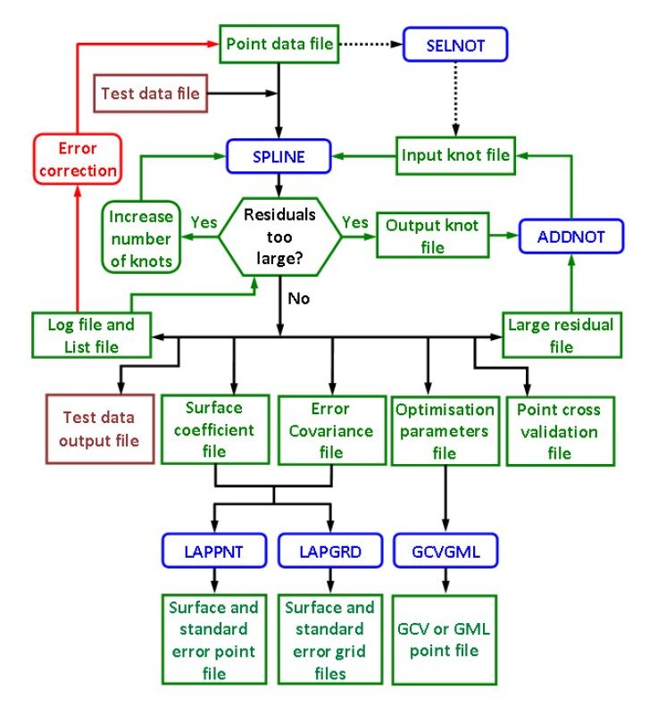
Main data flows
The flow chart below shows the main data flows through the programs described in the program summary. The overall analysis proceeds from point data to output point and grid files suitable for storage and plotting by a geographic information system (GIS) and other plotting packages. The analyses by SPLINA and SPLINB provide up to six output files which provide statistical analyses, support detection of data errors, an important phase of the analysis, and facilitate determination of additional knots by ADDNOT for the SPLINB program. The output surface coefficients and error covariance matrices enable systematic interrogation of the fitted surfaces by LAPPNT and LAPGRD. The GCV files output by AVGCVA and AVGCVB can also assist detection of data errors and revision of the specifications of the spline model.
See the ANUSPLIN data flow diagram for more information
Fitting climate surfaces
The surface fitting procedure was primarily developed for this task so that there are normally at least two independent spline variables, longitude and latitude, in this order and in units of decimal degrees. A third independent variable, elevation above sea-level, is often appropriate when fitting surfaces to temperature or precipitation. This is normally included as a third independent spline variable, in which case it should be scaled to be in units of kilometres. Minor improvements can sometimes be had by slightly altering this scaling of elevation. This scaling was originally determined by Hutchinson and Bischof (1983) and has been verified by Hutchinson (1995, 1998b).
Over restricted areas, superior performance can sometimes be achieved by including elevation not as an independent spline variable but as an independent covariate. Thus, in the case of fitting a temperature surface, the coefficient of an elevation covariate would be an empirically determined temperature lapse rate (Hutchinson, 1991a). Other factors which influence the climate variable may be included as additional covariates if appropriate parameterizations can be determined and the relevant data are available. These might include, for example, topographic effects other than elevation above sea-level. Other applications to climate interpolation have been described by Hutchinson et al. (1984ab, 1996a) and Hutchinson (1989a, 1991ab). Applications of fitted spline climate surfaces to global agroclimatic classifications and to the assessment of biodiversity are described by Hutchinson et al. (1992, 1996b).
To fit multi-variate climate surfaces, the values of the independent variables need only be known at the data points. Thus meteorological stations should be accurately located in position and elevation. Errors in these locations are often indicated by large values in the output ranked residual list. Recent applications have examined the utility of using elevation and slope and aspect obtained from digital elevation models of various horizontal resolutions (Hutchinson 1995, 1998b).
The LAPGRD program can be used to calculate a regular grids of fitted climate values and their standard errors, for mapping and other purposes, provided a regular grid of values of each independent variable, additional to longitude and latitude, is supplied. This usually means that a regular grid digital elevation model (DEM) is required. A technique for calculating such DEMs from elevation and stream line data has been described by Hutchinson (1988, 1989b, 1996).
References
- Bates D and Wahba G. 1982. Computational methods for generalised cross validation with large data sets. In: Baker CTH and Miller GF (eds). Treatment of Integral Equations by Numerical Methods. New York: Academic Press: 283-296.
- Bates D, Lindstrom M, Wahba G and Yandell B. 1987. GCVPACK - routines for generalised cross validation.Commun. Statist. B - Simulation and Computation 16: 263-297.
- Craven P and Wahba G. 1979. Smoothing noisy data with spline functions. Numerische Mathematik 31: 377-403.
- Dongarra, JJ., Moler, CB., Bunch, JR. and Stewart GW. 1979. LINPACK Users' Guide. SIAM, Philadelphia.
- Elden L. 1984. A note on the computation of the generalised cross-validation function for ill-conditioned least squares problems. BIT 24: 467-472.
- Hutchinson MF. 1984. A summary of some surface fitting and contouring programs for noisy data. CSIRO Division of Mathematics and Statistics, Consulting Report ACT 84/6. Canberra, Australia.
- Hutchinson MF. 1988. Calculation of hydrylogically sound digital elevation models. Third International Symposium on Spatial Data Handling. Columbus, Ohio: International Geographical Union: 117-133.
- Hutchinson MF. 1989a. A new objective method for spatial interpolation of meteorological variables from irregular networks applied to the estimation of monthly mean solar radiation, temperature, precipitation and windrun. CSIRO Division of Water Resources Tech. Memo. 89/5: 95-104.
- Hutchinson MF. 1989b. A new procedure for gridding elevation and stream line data with automatic removal of spurious pits. Journal of Hydrology 106: 211-232.
- Hutchinson MF. 1991a. The application of thin plate smoothing splines to continent-wide data assimilation. In:. Jasper JD (ed.) BMRC Research Report No.27, Data Assimilation Systems. Melbourne: Bureau of Meteorology: 104-113.
- Hutchinson MF. 1991b. Climatic analyses in data sparse regions. In:. Muchow RC and. Bellamy JA (eds).Climatic Risk in Crop Production, CAB International, 55-71.
- Hutchinson MF. 1993. On thin plate splines and kriging. In: Tarter ME and Lock MD.(eds). Computing and Science in Statistics 25. University of California, Berkeley: Interface Foundation of North America: 55-62.
- Hutchinson MF. 1995. Interpolating mean rainfall using thin plate smoothing splines. International Journal of GIS 9: 305-403.
- Hutchinson MF. 1996. A locally adaptive approach to the interpolation of digital elevation models. Third Conference/Workshop on Integrating GIS and Environmental Modeling. Santa Barbara: NCGIA, University of California.
- Hutchinson MF. 1998a. Interpolation of rainfall data with thin plate smoothing splines: I two dimensional smoothing of data with short range correlation. Journal of Geographic Information and Decision Analysis2(2): 152-167.
- Hutchinson MF. 1998b. Interpolation of rainfall data with thin plate smoothing splines: II analysis of topographic dependence. Journal of Geographic Information and Decision Analysis 2(2): 168-185.
- Hutchinson MF. and Bishof RJ. 1983. A new method for estimating the spatial distribution of mean seasonal and annual rainfall applied to the Hunter Valley, New South Wales. Australian Meteorological Magazine 31: 179-184.
- Hutchinson MF, Booth TH, Nix HA and McMahon JP. 1984a. Estimating monthly mean values of daily total solar radiation for Australia. Solar Energy 32: 277-290.
- Hutchinson MF., Kalma JD and Johnson ME. 1984b. Monthly estimates of wind speed and wind run for Australia. Journal of Climatology 4: 311-324.
- Hutchinson MF. and de Hoog FR. 1985. Smoothing noisy data with spline functions. Numerische Mathematik 47: 99-106.
- Hutchinson MF. Nix HA. and McMahon JP. 1992. Climate constraints on cropping systems. In: Pearson CJ. (ed), Ecosystems of the World, 18 Field Crop Ecosystems. Amsterdam: Elsevier: 37-58.
- Hutchinson MF. and Gessler PE. 1994. Splines - more than just a smooth interpolator. Geoderma 62: 45-67.
- Hutchinson MF. Nix HA, McMahon JP. and Ord KD. 1996a. The development of a topographic and climate database for Africa. In: Proceedings of the Third International Conference/Workshop on Integrating GIS and Environmental Modeling, NCGIA, Santa Barbara, California.
- Hutchinson MF., Belbin L., Nicholls AO., Nix HA., McMahon J.P. and Ord KD. 1996b. Rapid Assessment of Biodiversity, Volume Two, Spatial Modelling Tools. The Australian BioRap Consortium, Australian National University, 142pp.
- Kesteven JL. and Hutchinson MF. 1996. Spatial modelling of climatic variables on a continental scale. In: Proceedings of the Third International Conference/Workshop on Integrating GIS and Environmental Modeling, NCGIA, Santa Barbara, California.
- Schimek, M.G. (ed.) 2000. Smoothing and regression: approaches, computation and application. John Wiley & Sons. New York.
- Silverman BW. 1985. Some aspects of the spline smoothing approach to nonparametric regression curve fitting (with discussion). Journal Royal Statistical Society Series B 47: 1-52.
- Wahba G. 1979. How to smooth curves and surfaces with splines and cross-validation. Proc. 24th Conference on the Design of Experiments. US Army Research Office 79-2, Research Triangle Park, NC: 167-192.
- Wahba G. 1983. Bayesian confidence intervals for the cross-validated smoothing spline. Journal Royal Statistical Society Series B 45: 133-150.
- Wahba G. 1990. Spline Models for Observational Data. CBMS-NSF Regional Conference Series in Applied Mathematics 59, SIAM, Philadelphia, Pennsylvania.